Flux: The Flexible Machine Learning Framework for Julia
With Julia jumping up the ranks as one of the most loved languages in this year’s Stack Overflow Developer survey and JuliaCon 2020 kicking off in the next few days, I thought this might be a good time to talk about machine learning in Julia. In this post, we’ll touch on Julia and some of its more interesting features before moving on to talk about Flux, a pure-Julia machine learning framework. By comparing a simple MNIST classifier in Flux to the equivalent Pytorch and Tensorflow 2 implementations, we begin to get an idea of the strengths and fun quirks of doing machine learning in Flux.
The Julia Language
The founders of Julia were looking to create a language which was geared towards interactive scientific computing, whilst at the same time supporting more advanced software engineering processes via direct JIT-compilation to native code. To facilitate this dual-purpose, Julia uses dynamic typing with the default behaviour being to allow values of any type when no type specification is provided. Further expressiveness is permissible in Julia via optional typing which provides some of the efficiency gains typically associated with static languages. Having spent my formative programming years writing C++ code, and now almost exclusively working in Python, the option to type my machine learning code is incredibly appealing.
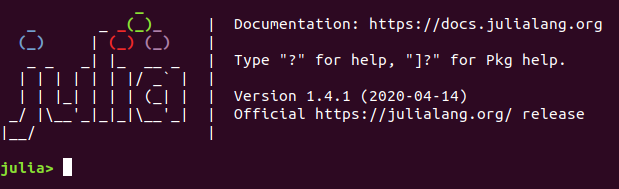
The REPL interactive prompt has several great features, such as built-in help (which you can get to by simply typing ?) or the built-in package manager (which can be accessed via ]).
One of the advantages of Julia is that it supports multiple dispatch, a paradigm which means that we never need to know argument types before passing them into a method. This allows us to write generic algorithms which can be easily re-used - a property which makes an open-source machine learning framework, like Flux, an enticing prospect. Stefan Karpinski elegantly contrasts this behaviour with single-dispatch object-orientated languages like C++ in his talk, The Unreasonable Effectiveness of Multiple Dispatch.
If you’re interested in the Julia language in general, I’d recommend watching this interview with two of the co-founders, Viral Shah and Jeff Bezanson.
The Magic of Flux
Flux is a fairly young framework with the first commit made in 2016. Consequentially it has been built with modern deep learning architectures in mind. Sequential layers can be chained together with ease, the Zygote.jl dependency takes care of automatic differentiation, and full GPU support is provided by CUDA.jl, all the while keeping the Flux code-base to a fraction of the size of PyTorch and Tensorflow.
To showcase the framework, we compare two Flux implementations of the typical MNIST digit classifier to their Tensorflow and Pytorch equivalents. If you just want to jump straight into the full scripts, have a look at my Github repository.
Functional Comparison: Flux vs Tensorflow
With Tensorflow being the most widely used deep learning framework in industry, it is worth comparing the Flux API to the Tensorflow functional API.
Model Definition
In Flux, we build sequential models by simply chaining together a series of Flux layers. This is demonstrated below where we construct a feed-forward network of two dense layers which follow on from a simple flattening layer. A typical ReLU activation is used in the hidden layer along with dropout for regularisation. This is all neatly wrapped up in a Julia function for us to use in our script.
function create_model(input_dim, dropout_ratio, hidden_dim, num_classes)
    return Chain(
        Flux.flatten,
        Dense(input_dim, hidden_dim, relu),
        Dropout(dropout_ratio),
        Dense(hidden_dim, num_classes)
    )
end
In Tensorflow 2, the recommended method for building eager models is to use the functional Keras API. In the snippet below, we see the equivalent code looks incredibly similar to the Flux implementation.
def create_model(input_dims, dropout_ratio, hidden_dim, num_classes):
    return tf.keras.models.Sequential([
        tf.keras.layers.Flatten(input_shape=input_dims),
        tf.keras.layers.Dense(hidden_dim, activation='relu'),
        tf.keras.layers.Dropout(dropout_ratio),
        tf.keras.layers.Dense(num_classes)
    ])
Dataloaders
Before we can start training these models, the MNIST data needs to be collated in an easily ingestible way. The Flux.Data module has a special Dataloader type which handles batching, iteration, and shuffling over the data. Combined with the onehotbatch function, this makes generating loaders for the training and test set data pretty straightforward. Notice that in this function, the optional typing of function arguments is showcased.
function get_dataloaders(batch_size::Int, shuffle::Bool)
    train_x, train_y = MNIST.traindata(Float32)
    test_x, test_y = MNIST.testdata(Float32)
    train_y, test_y = onehotbatch(train_y, 0:9), onehotbatch(test_y, 0:9)

    train_loader = DataLoader(
        train_x, train_y, batchsize=batch_size, shuffle=shuffle)
    test_loader = DataLoader(
        test_x, test_y, batchsize=batch_size, shuffle=shuffle)

    return train_loader, test_loader
end
Since MNIST is a simple and small dataset, for the purposes of this demonstration a straightforward implementation for collating the data in Tensroflow is used.
def get_data():
    mnist = tf.keras.datasets.mnist
    (x_train, y_train), (x_test, y_test) = mnist.load_data()
    x_train, x_test = x_train / 255.0, x_test / 255.0
    return x_train, y_train, x_test, y_test
Training Loop
At the start of the main function, we create the dataloaders and instantiate the model. The trainable parameters, which will be passed to the train function, are collected into an object using Flux.params(model). Flux offers several optimisers such as RMSProp, ADADelta, and AdaMax, but in this demonstration ADAM is used. Notice that the learning rate is set using the unicode character η. Simply being able to drop unicode characters into any Julia code is a great feature which makes Flux implementations look closer to the mathematical model as published in the original article or journal. The instantiation of the optimiser is followed by the loss function definition, which thanks to the concise Julia syntax, also exhibits a neat mathematical quality. The choice of logitcrossentropy (which applies the softmax function to the logit output internally) is commonly used as a more stable alternative to crossentropy in classification problems.
All four of the above-mentioned components come together in the Flux.train! loop, which optimises trainable parameters given the loss function, optimiser, and the training dataloader. The loop is run a number of times using the @epochs macro. Notice that the model is contained in the loss function definition and so it does not need to be passed in explicitly. We simply indicate which parameters we want to be optimised.
function main(num_epochs, batch_size, shuffle, η)
    train_loader, test_loader = get_dataloaders(batch_size, shuffle)

    model = create_model(28*28, 0.2, 128, 10)
    trainable_params = Flux.params(model)

    optimiser = ADAM(η)
    loss(x,y) = logitcrossentropy(model(x), y)

    @epochs num_epochs Flux.train!(
        loss, trainable_params, train_loader, optimiser)
end
The Tensorflow implementation has a similar flow. The data is loaded, model initialised, and the loss function defined. Unlike in the Flux implementation, the model is not present in the loss function. Tensorflow builds the computational graph at the point of calling compile on the model and only executes after calling fit.
def main(num_epochs, optimiser):
    x_train, y_train, x_test, y_test = get_data()

    model = create_model(
        input_dims=(28, 28),
        hidden_layer_dim=128,
        dropout_ratio=0.2,
        num_classes=10
    )

    loss = tf.keras.losses.SparseCategoricalCrossentropy(from_logits=True)

    model.compile(
        optimizer=optimiser,
        loss=loss,
        metrics=['accuracy']
    )

    model.fit(x_train, y_train, epochs=num_epochs)
Evaluation
Once the models have been trained, running evaluation on the training and test sets is a natural next step. In this case, the classification accuracy is selected as the metric to judge model performance. A quick helper function is defined in Julia for this purpose.
function accuracy(data_loader, model)
    acc_correct = 0
    for (x, y) in data_loader
        batch_size = size(x)[end]
        acc_correct += sum(onecold(model(x)) .== onecold(y)) / batch_size
    end
    return acc_correct / length(data_loader)
end
The following code snippet is inserted directly after training the model in the main function above. The first step puts the model into evaluation mode, which has the effect of turning off dropout in our Flux model. This is imperative for ensuring that the Flux model behaves as expected during inference and validation. The accuracy helper function is then used to generate accuracies for the training and test data.
    # Later in `main(..)`
    testmode!(model)
    @show accuracy(train_loader, model)
    @show accuracy(test_loader, model)
Fortunately for the Tensorflow implementation, the accuracy metric was already compiled with the model. As a result, evaluation results are trivially computed using model.evaluate.
    # Later in `main(..)`
    print('Evaluate on training data')
    model.evaluate(x_train, y_train, verbose=2)
    print('Evaluate on test data')
    model.evaluate(x_test, y_test, verbose=2)
Module-based Comparison: Flux vs PyTorch
In addition to the functional API, Flux supports a modular approach to building models as well. This section demonstrates how to build an equivalent model to those presented above using custom training loops and modular model design. Rather than comparing to Tensorflow again, this time the corresponding PyTorch code is used as the basis of comparison.
PyTorch Helper Functions
To start off, a PyTorch dataloading function is set up using the built-in dataloader class.
def get_dataloaders(batch_size, shuffle):
    transform = transforms.Compose([
        transforms.ToTensor(),
        transforms.Normalize((0.1307,), (0.3081,))
    ])

    training_set = datasets.MNIST(
        '../data', train=True, transform=transform, download=True)
    test_set = datasets.MNIST(
        '../data', train=False, transform=transform)

    train_loader = torch.utils.data.DataLoader(
        training_set, batch_size=batch_size, shuffle=shuffle)
    test_loader = torch.utils.data.DataLoader(
        test_set, batch_size=batch_size, shuffle=shuffle)

    return train_loader, test_loader
We also define an accuracy function to be used during evaluation.
def accuracy(model, test_loader, batch_size):
    model.eval()
    correct = 0.0
    with torch.no_grad():
        for batch_x, batch_y in test_loader:
            pred_batch = model(batch_x)
            pred_batch = pred_batch.argmax(dim=1, keepdim=True)
            correct += pred_batch.eq(batch_y.view_as(pred_batch)).sum().item()

    return correct / (len(test_loader) * batch_size)
The Modular Model
The feedforward network is defined using a struct type where each layer is an attribute. The arguments passed to the new(..) function in the inner constructor are set to the corresponding object attributes using their relative order. In contrast to the functional definition, the layers are not chained together. Therefore the forward pass behaviour is required to be defined explicitly. An anonymous function, used in a similar way as the __call__ function in Python, is defined for this purpose. Any object of type FFNetwork can re-use the forward pass implementation. In the hypothetical scenario where another model class is defined in the same script with its own anonymous forward pass function, the multiple dispatch paradigm would handle passing the instance to the appropriate forward pass function at runtime.
struct FFNetwork
    fc_1
    dropout
    fc_2
    FFNetwork(
        input_dim::Int, hidden_dim::Int, dropout::Float32, num_classes::Int
    ) = new(
        Dense(input_dim, hidden_dim, relu),
        Dropout(dropout),
        Dense(hidden_dim, num_classes),
    )
end

function (net::FFNetwork)(x)
    x = Flux.flatten(x)
    return net.fc_2(net.dropout(net.fc_1(x)))
end
The PyTorch class definition inherits from the torch.nn.Module base class which provides it with built-in functionality such as being able to easily move the model onto a GPU via to(..), amongst others. In contrast to the relationship observed above, the forward pass definition for each class is built into the class definition. This means that the only way to re-use that code would be via some inheritance structure. This can very quickly lead to complicated inheritance patterns which force the class definitions to take on more complexity than would otherwise be required.
class FFNetwork(Module):
    def __init__(self, input_dims, hidden_dim, dropout_ratio, num_classes):
        super(FFNetwork, self).__init__()
        self.flat_image_dims = np.prod(input_dims)
        self.fc_1 = torch.nn.Linear(self.flat_image_dims, hidden_dim)
        self.dropout = torch.nn.Dropout(dropout_ratio)
        self.fc_2 = torch.nn.Linear(hidden_dim, num_classes)

    def forward(self, x):
        x = x.view(-1, self.flat_image_dims)
        return self.fc_2(self.dropout(F.relu(self.fc_1(x))))
Custom Training Loops
Flux permits custom training loops to enable more sophisticated metric tracking and loss formulations. The trade-off with this approach is that it requires more work on the software side. For each batch in each epoch, the loss is manually accumulated and the model parameters updated. The pullback(..) function, imported from Zygote, automatically calculates the loss and returns a pullback, which can be used to obtain the gradients for all trainable parameters by passing in 1f0. A difference to note is that modular Flux models require that each trainable layer must be specifically passed into the params function rather than simply passing the full chained functional model. Although this classification example is rather simple and does not take full advantage of the explicit pullback call, models such as GANs and VAEs benefit greatly from the increased flexibility.
function cross_entropy_loss(model, x, y)
    ŷ = model(x)
    return logitcrossentropy(model(x), y)
end

function main(num_epochs, batch_size, shuffle, η)
    train_loader, test_loader = get_dataloaders(batch_size, shuffle)

    model = FFNetwork(28*28, 128, 0.2f0, 10)
    trainable_params = Flux.params(model.fc_1, model.fc_2)
    optimiser = ADAM(η)

    for epoch = 1:num_epochs
        acc_loss = 0.0
        for (x_batch, y_batch) in train_loader
            loss, back = pullback(trainable_params) do
                cross_entropy_loss(model, x_batch, y_batch)
            end
            gradients = back(1f0)
            Flux.Optimise.update!(optimiser, trainable_params, gradients)
            acc_loss += loss
        end
        avg_loss = acc_loss / length(train_loader)
        println("Epoch: $epoch - loss: $avg_loss")
    end
end
Similarly, the PyTorch implementation requires a more granular treatment of the training loop. In train_epoch the average loss over the full epoch is accumulated and returned. For each batch, gradients are obtained by calling backwards() on the loss object returned from the cross entropy loss function. The model parameters are then updated using optimiser.step() and gradients are reset to zero using optimiser.zero_grad(). Overall the Flux and PyTorch custom training loops have a very similar feel with the key difference being that in PyTorch the gradients are required to be reset to zero manually, while in Flux each layer with trainable parameters needs to be explicitly provided to the pullback function.
def train_epoch(model, train_loader, optimiser):
    loss = torch.nn.CrossEntropyLoss()
    acc_loss = 0.0
    model.train()
    for batch_x, batch_y in train_loader:
        optimiser.zero_grad()
        pred_batch = model(batch_x)
        train_loss = loss(pred_batch, batch_y)
        train_loss.backward()
        optimiser.step()
        acc_loss += train_loss.item()
    return acc_loss / len(train_loader)

def main(num_epochs, batch_size, shuffle):
    train_loader, test_loader = get_dataloaders(batch_size, shuffle)

    model = FFNetwork(
        input_dims=(28, 28),
        hidden_dim=128,
        dropout_ratio=0.2,
        num_classes=10
    )
    optimiser = Adam(model.parameters())

    for epoch_idx in range(num_epochs):
        loss = train_epoch(model, train_loader, optimiser)
        print(f'Epoch {epoch_idx + 1} loss: {loss}')
Evaluation is unchanged in the modular Flux implementation. In PyTorch we simply call the accuracy helper function defined above.
train_acc = accuracy(model, train_loader, batch_size)
test_acc = accuracy(model, test_loader, batch_size)
print(f'train_acc: {train_acc}  -  test_acc: {test_acc}')
Final Thoughts
Flux provides enough functionality and readability to make it an interesting competitor to the two more established machine learning frameworks. From a personal perspective, I think that Flux is a fantastic option for research projects and a much-needed break from the monotony of Python in my machine learning life. I’m quite excited about Flux’s progress over the last few years and I am certainly hoping to see more tools and papers publishing their work in Flux - particularly in NLP. From an industry user perspective, the sheer extent to which PyTorch and Tensorflow have been battle-tested makes them a more reliable option which continues to have more off-the-shelf functionality and pre-trained models than Flux.
To cite this post:
@article{kastanos20fluxml,
  title   = "Flux: The Flexible Machine Learning Framework for Julia",
  author  = "Alexandros Kastanos",
  journal = "alecokas.github.io",
  year    = "2020",
  url     = "https://alecokas.github.io/julia/flux/2020/07/20/flux-flexible-ml-for-julia.html"
}
References
[1] Innes, Mike. “Flux: Elegant machine learning with Julia.” Journal of Open Source Software 3.25 (2018): 602.
[2] Bezanson, Jeff, et al. “Julia: A fresh approach to numerical computing.” SIAM review 59.1 (2017): 65-98.
[3] Paszke, Adam, et al. “Automatic differentiation in pytorch.” (2017).
[4] Abadi, Martín, et al. “Tensorflow: Large-scale machine learning on heterogeneous distributed systems.” arXiv preprint arXiv:1603.04467 (2016).
[5] LeCun, Yann, Corinna Cortes, and C. J. Burges. “MNIST handwritten digit database.” (2010): 18.