Convolutional VAE in Flux
In this post, we’ll take a look at variational autoencoders and demonstrate an implementation using the FashionMNIST dataset and Flux. This content follows on from my previous post where I introduce Flux and show how it compares with Tensorflow and PyTorch.
Formulating the Variational Autoencoder
Before looking at the implementation, I’ll present a short overview of autoencoders and the differentiating features of a variational autoencoder (VAE). For a more complete description of the background and the loss function derivation, have a look at the original VAE paper: Auto-Encoding Variational Bayes.
Autoencoders
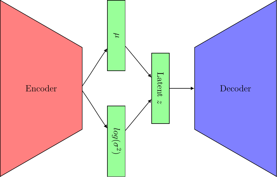
An autoencoder is a type of neural network made up of two principal components, an encoder and a decoder. The role of the encoder is to extract learnt features from the input data, \(x\), and represent them in a constrained latent space, \(z\). Ideally, this latent space, sometimes called the bottleneck layer, is a representation of the compressed underlying characteristics of the data. The decoder then generates a reconstruction of the original image, \(\hat{x}\), which aims to closely resemble the input data. If the encoder and decoders are modelled using neural networks, we can train the autoencoder to minimise the reconstruction loss between \(x\) and \(\hat{x}\).
Making them Variational
The key difference between the vanilla autoencoder, and a VAE, is in the treatment of the latent space, \(z\). For VAEs we model the latent space as a probability distribution, \(q(z|x)\), which approximates some prior, \(p(z)\). Typically this prior is the Gaussian \(\mathcal{N} (0, 1)\). We train the encoder to learn the mean and standard deviation of \(q(z | x)\), which we then use to generate samples to feed into the decoder network. Since we still want to train our VAE using backpropagation and gradient descent, we need a mechanism for removing the sampling operation from the backprogation path whilst still obtaining samples of \(z\). To this end, we apply the reparameterisation trick and perform our sampling via \(z \sim \mu + \sigma \odot \epsilon\) where \(\epsilon \sim p(z)\).
As before, we define our loss function such that we minimise the reconstruction loss between the original \(x\) and the reconstruction \(\hat{x}\). An additional KL loss term is included which penalises the model when \(q(z | x)\) deviates from \(p(z)\). This loss function ends up being equivalent to the Evidence Lower Bound (ELBO), which during optimisation we intent to maximise. If we parameterise our encoder and decoder with the parameters \(\phi\) and \(\theta\) respectively, the objective can be written as follows.
Building the VAE in Flux
For the remainder of this post, we move away from the theory and step through an example implementation of a Convolutional VAE using Flux. The code snippets to follow are taken from my Github repository, so head over there if you want to simply jump to the complete scripts. Let’s get started with learning how to leverage dataloaders to easily import the FashionMNIST dataset.
Loading the FashionMNIST dataset
FashionMNIST is an incredibly popular benchmarking dataset, made up of low-resolution greyscale images of clothes and accessories, which operates as an easy drop-in replacement for the simpler original MNIST dataset. Each image is one of 10 possible item types, which are used as the 10 labelled classes. The full dataset, established by Zalando, is made up of a training set of 60 000 images and a test set of 10 000 images, where all images are 28 by 28 in pixel dimensions. For our demonstration, we zero-pad each image to 32 by 32 pixels so that we can apply a similar model architecture as documented in β-VAE: Learning Basic Visual Concepts with a Constrained Variational Framework and Understanding disentangling in β-VAE.
We can define a function to do just that, and return a Flux.Data.DataLoader object which will handle the batching and shuffling of our data.
function get_train_loader(batch_size, shuffle::Bool)
    # FashionMNIST is made up of 60k 28 by 28 greyscale images
    train_x, train_y = FashionMNIST.traindata(Float32)
    train_x = reshape(train_x, (28, 28, 1, :))
    train_x = parent(padarray(train_x, Fill(0, (2,2,0,0))))
    return DataLoader(
        train_x, train_y, batchsize=batch_size, shuffle=shuffle, partial=false
    )
end
Defining the model
Next, we have a method which defines a fairly typical Convolutional VAE architecture. The encoder is defined by chaining 3 convolutional layers, with a kernel width of 4 and 32 filters. The output from these layers is then flattened before being pushed to two dense layers with 256 neurons each. This portion of the encoder which we call encoder_features has two separate fully connected layers branching off it to provide us with the networks which generate the mean (\(\mu\)) and logarithmic variance (\(log\sigma^2\)) vectors. We use the log variance, rather than the variance, so that we can leave the encoder_logvar network unconstrained and not worry about how forcing the network to only produce positive values might affect the optimisation process.
The decoder is defined to look like the transpose of the encoder where we expect the input from the latent space, \(z\), to have the same dimensionality of the \(\mu\) vector produced by the encoder. Something important to note in the decoder is that we have defined a custom layer Reshape rather than using the operation x -> reshape(x, (4, 4, 32, :)). This custom layer is able to be saved and loaded using the BSON package while the built-in reshape operation caused problems when I tried to forward pass a model loaded from disk.
struct Reshape
    shape
end
Reshape(args...) = Reshape(args)
(r::Reshape)(x) = reshape(x, r.shape)
Flux.@functor Reshape ()

function create_vae()
    # Define the encoder and decoder networks
    encoder_features = Chain(
        Conv((4, 4), 1 => 32, relu; stride = 2, pad = 1),
        Conv((4, 4), 32 => 32, relu; stride = 2, pad = 1),
        Conv((4, 4), 32 => 32, relu; stride = 2, pad = 1),
        Flux.flatten,
        Dense(32 * 4 * 4, 256, relu),
        Dense(256, 256, relu)
    )
    encoder_μ = Chain(encoder_features, Dense(256, 10))
    encoder_logvar = Chain(encoder_features, Dense(256, 10))

    decoder = Chain(
        Dense(10, 256, relu),
        Dense(256, 256, relu),
        Dense(256, 32 * 4 * 4, relu),
        Reshape(4, 4, 32, :),
        ConvTranspose((4, 4), 32 => 32, relu; stride = 2, pad = 1),
        ConvTranspose((4, 4), 32 => 32, relu; stride = 2, pad = 1),
        ConvTranspose((4, 4), 32 => 1; stride = 2, pad = 1)
    )
    return encoder_μ, encoder_logvar, decoder
end
The training loop
Flux facilitates custom training loops, which are great for allowing custom progress tracking and metric logging code. The train() function below takes in the three Chain components which make up our VAE, the dataloader described above, as well as some key training parameters. These include a weight decay regularisation parameter (\(\lambda\)), a hyperparameter which controls the relative importance of disentangling factors of variation (\(\beta\)), amongst others. For each batch, we calculate the loss as defined in vae_loss() and generate a pullback from which to calculate the gradients.
function train(
    encoder_μ, encoder_logvar, decoder, dataloader,
    num_epochs, λ, β, optimiser, save_dir)
    trainable_params = Flux.params(encoder_μ, encoder_logvar, decoder)

    for epoch_num = 1:num_epochs
        acc_loss = 0.0
        progress_tracker = Progress(
            length(dataloader), 1,
            "Training epoch $epoch_num: "
        )
        for (x_batch, y_batch) in dataloader
            # pullback(..) returns the loss and a pullback operator (back)
            loss, back = pullback(trainable_params) do
                vae_loss(encoder_μ, encoder_logvar, decoder, x_batch, β, λ)
            end
            # Feed the pullback 1 to obtain the gradients
            gradients = back(1f0)
            Flux.Optimise.update!(optimiser, trainable_params, gradients)
            if isnan(loss)
                break
            end
            acc_loss += loss
            next!(progress_tracker; showvalues=[(:loss, loss)])
        end
        avg_loss = acc_loss / length(dataloader)
        metrics = DataFrame(epoch=epoch_num, negative_elbo=avg_loss)
        println(metrics)
        CSV.write(
            joinpath(save_dir, "metrics.csv"), metrics,
            header=(epoch_num==1), append=true)
        save_model(encoder_μ, encoder_logvar, decoder, save_dir, epoch_num)
    end
    println("Training complete!")
end
Calculating the loss
Before we can train our model, we need to define the loss function vae_loss(). The method takes in our mean and logvar encoders, the decoder, the batch of images to train on, \(x\), as well as the \(\beta\) and \(\lambda\) hyperparameters. First, \(x\) is fed through the encoder to generate our mean and log variance vectors. We then sample from \(q(z|x)\) using the reparameterisation trick, where we obtain the standard deviation through log manipulation, to obtain \(z\). The reconstructed image is then generated by pushing \(z\) through the decoder. The ELBO is calculated by subtracting the reverse KL divergence from the negative reconstriction loss. Finally, the function returns the sum of the negative ELBO and an \(L_{2}\) weight decay regularisation term. As mentioned above, we actually want to maximise the ELBO, but in the context of a code implementation, it is more intuitive to minimise the negative ELBO.
function vae_loss(encoder_μ, encoder_logvar, decoder, x, β, λ)
    batch_size = size(x)[end]
    @assert batch_size != 0

    # Forward propagate through mean encoder and std encoders
    μ = encoder_μ(x)
    logvar = encoder_logvar(x)
    # Apply reparameterisation trick to sample latent
    z = μ + randn(Float32, size(logvar)) .* exp.(0.5f0 * logvar)
    # Reconstruct from latent sample
    x̂ = decoder(z)
    # Negative reconstruction loss Ε_q[logp_x_z]
    logp_x_z = -sum(logitbinarycrossentropy.(x̂, x)) / batch_size
    # KL(qᵩ(z|x)||p(z)) where p(z)=N(0,1) and qᵩ(z|x) models the encoder
    # The @. macro makes sure that all operates are elementwise
    kl_q_p = 0.5f0 * sum(@. (exp(logvar) + μ^2 - logvar - 1f0)) / batch_size
    # Weight decay regularisation term
    reg = λ * sum(x->sum(x.^2), Flux.params(encoder_μ, encoder_logvar, decoder))
    # We want to maximise the evidence lower bound (ELBO)
    elbo = logp_x_z - β .* kl_q_p
    # So we minimise the sum of the negative ELBO and a weight penalty
    return -elbo + reg
end
Evaluate a trained model
That is the main modelling done! For demonstration purposes, I trained the model for 10 epochs, using Flux’s Adam optimiser with a learning rate of 0.0001, and saved it to disk. Before we can have a look at some images, let’s define a test data loader (which is very similar to the training data loader) and a function to save our images to disk.
function get_test_loader(batch_size, shuffle::Bool)
    # The FashionMNIST test set is made up of 10k 28 by 28 greyscale images
    test_x, test_y = FashionMNIST.testdata(Float32)
    test_x = reshape(test_x, (28, 28, 1, :))
    test_x = parent(padarray(test_x, Fill(0, (2,2,0,0))))
    return DataLoader(test_x, test_y, batchsize=batch_size, shuffle=shuffle)
end

function save_to_images(x_batch, save_dir::String,
                        prefix::String, num_images::Int64)
    @assert num_images <= size(x_batch)[4]
    for i=1:num_images
        save(joinpath(save_dir, "$prefix-$i.png"),
             colorview(Gray, permutedims(x_batch[:,:,1,i], (2, 1))))
    end
end
Additionally, we define a function to pass images through the VAE to reconstruct images from the unseen test set. A key thing to note is that we apply the sigmoid activation to the reconstructed images so that they are normalised appropriately.
function reconstruct_images(encoder_μ, encoder_logvar, decoder, x)
    # Forward propagate through mean encoder and std encoders
    μ = encoder_μ(x)
    logvar = encoder_logvar(x)
    # Apply reparameterisation trick to sample latent
    z = μ + randn(Float32, size(logvar)) .* exp.(0.5f0 * logvar)
    # Reconstruct from latent sample
    x̂ = decoder(z)
    return sigmoid.(x̂)
end
Now there is nothing left to do than load the trained VAE from disk, and set up a loop where we reconstruct test set images to compare with the originals.
function load_model(load_dir::String, epoch::Int)
    print("Loading model...")
    load_path = joinpath(load_dir, "model-$epoch.bson")
    @load load_path encoder_μ encoder_logvar decoder
    println("Done")
    return encoder_μ, encoder_logvar, decoder
end

function visualise()
    batch_size = 64
    shuffle = true
    num_images = 8
    epoch_to_load = 10

    encoder_μ, encoder_logvar, decoder = load_model("results", epoch_to_load)
    dataloader = get_test_loader(batch_size, shuffle)

    for (x_batch, y_batch) in dataloader
        save_to_images(x_batch, "results", "test-image", num_images)
        x̂_batch = reconstruct_images(
            encoder_μ, encoder_logvar, decoder, x_batch
        )
        save_to_images(x̂_batch, "results", "reconstruction", num_images)
        break
    end
end
Show me some images!
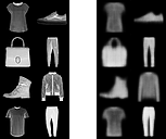
The two side-by-side images below demonstrate the reconstruction ability of the VAE on unseen data after training for 10 epochs. The set of images on the left are taken from the test set, while the images on the right are generated from the model. We see that the model has learnt a good enough latent representation to reconstruct the original samples to a reasonable degree of accuracy. That being said, the reconstructed images are certainly blurrier than the corresponding original images. This is a common problem in VAEs, which due to the reverse KL term in their objective exhibit zero-forcing properties and therefore suffer from over-dispersion.
Other VAEs
It is worth mentioning that there have been numerous variations on the VAE architecture. Some interesting examples include β-VAE, \(JS^{G_α}\)-VAEs, and NVAE. Furthermore, if you are specifically interested in disentangling in VAE, take a look at this work I was involved in where we investigated and contrasted a number of disentangling VAE architectures.
To cite this post:
@article{kastanos20fluxvae,
  title   = "Convolutional VAE in Flux",
  author  = "Alexandros Kastanos",
  journal = "alecokas.github.io",
  year    = "2020",
  url     = "http://alecokas.github.io/julia/flux/vae/2020/07/22/convolutional-vae-in-flux.html"
}
References
[1] Innes, Mike. “Flux: Elegant machine learning with Julia.” Journal of Open Source Software 3.25 (2018): 602.
[2] Kingma, Diederik P., and Max Welling. “Auto-encoding variational bayes.” arXiv preprint arXiv:1312.6114 (2013).
[3] Burgess, Christopher P., et al. “Understanding disentangling in $\beta$-VAE.” arXiv preprint arXiv:1804.03599 (2018).
[4] Higgins, Irina, et al. “beta-vae: Learning basic visual concepts with a constrained variational framework.” (2016).
[5] Zhang, Mingtian, et al. “Variational f-divergence minimization.” arXiv preprint arXiv:1907.11891 (2019).
[6] Deasy, Jacob, Nikola Simidjievski, and Pietro Liò. “Constraining Variational Inference with Geometric Jensen-Shannon Divergence.” arXiv preprint arXiv:2006.10599 (2020).
[7] Vahdat, Arash, and Jan Kautz. “NVAE: A Deep Hierarchical Variational Autoencoder.” arXiv preprint arXiv:2007.03898 (2020).